1Department of Mathematics and Statistics, Boston University2Howard Hughes Medical Institute, Janelia Research Campus3Departments of Physiology and Psychiatry, University of California, San Francisco4Kavli Institute for Fundamental Neuroscience, University of California, San Francisco5Howard Hughes Medical Institute, University of California, San Francisco*Corresponding author:
eric.denovellis@ucsf.edu
A state-space decoder combines what past spikes predict about a latent state with what
the newest spike says. We check, spike by spike, whether these two sources of information
point to overlapping regions of the state space. The result is analogous to a local,
time-resolved goodness-of-fit test: it can show when a decoding model fails and
suggest which of its assumptions is responsible.
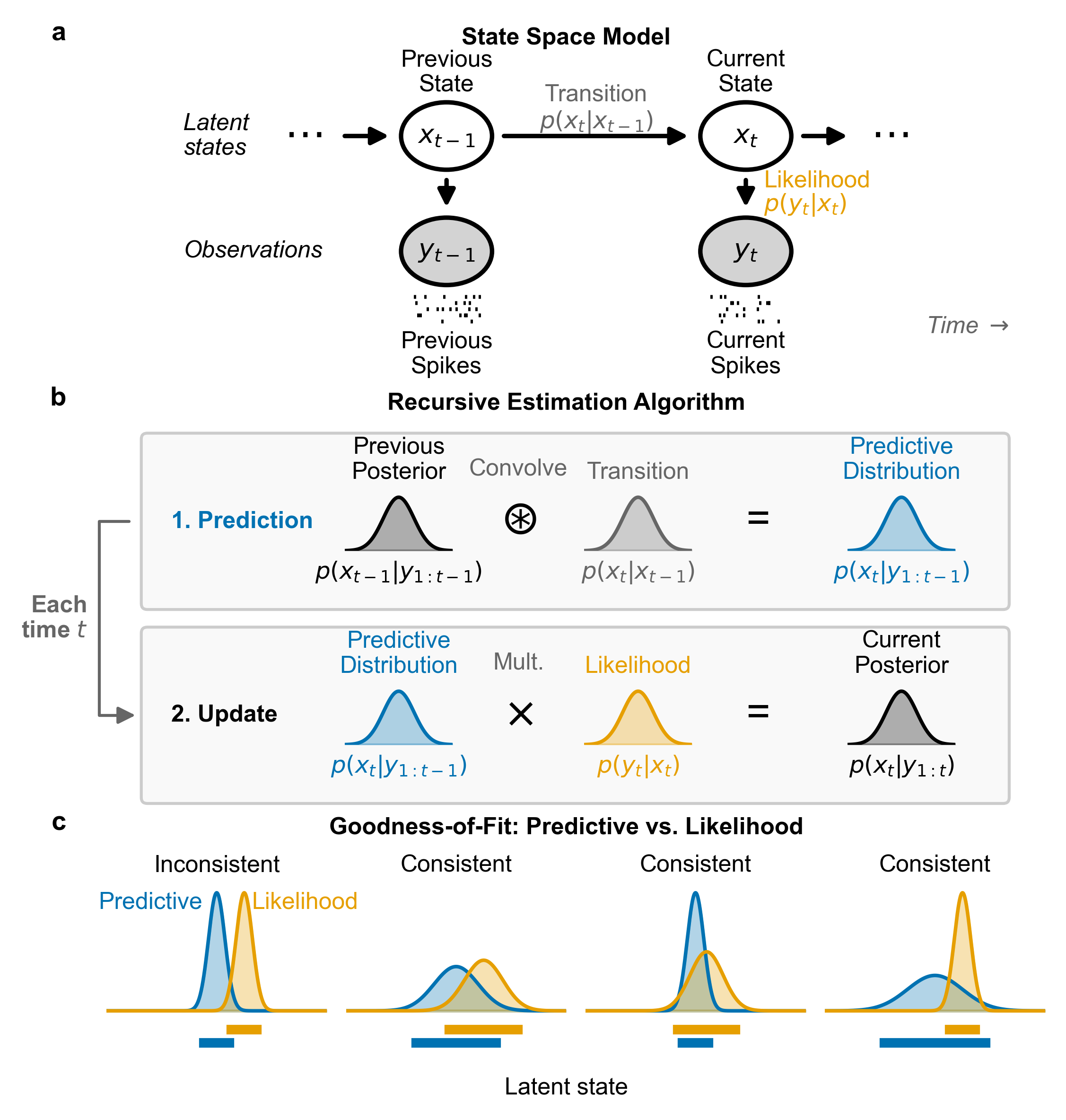
Figure 1 of the paper. (a) A state-space model links a latent state
to neural observations. (b) At each step the filter turns the previous posterior into a
one-step prediction, then multiplies it by the likelihood of the new spikes. (c) We
compare the prediction with each spike's likelihood. They are inconsistent when their
high-probability regions are mostly disjoint, and consistent when those regions overlap,
even if the two differ in center or spread.
Why local goodness-of-fit?
State-space models relate high-dimensional neural activity to low-dimensional latent
states, such as the position represented by hippocampal activity. Those states cannot be
observed, so a decoder cannot be checked against ground truth. The usual validation
tools, cross-validation and shuffle tests, summarize a whole recording in one number:
they say whether a model beats chance or a simpler alternative, but not when
during a session it fits poorly or which of its components is responsible.
Interpretable models are simplified on purpose. A place-cell decoder that ignores
momentum or bursting can still produce scientifically useful trajectories. Rather than
accept or reject such a model wholesale, we look inside it. At every spike, the filter
already holds two distributions over the latent state: the prediction,
which carries forward everything learned from past spikes, and the
likelihood of the newest spike. We ask whether they are consistent.
Prediction and likelihood
The decoder is a recursive Bayesian filter, the cycle in Figure 1b. It keeps a
posterior, its probability distribution over position given every spike
so far, and advances it one time step at a time in two moves. First it
predicts: the animal may have moved since the last step, so a movement
model spreads the posterior into the prediction P(x). Then it
updates: it multiplies the prediction by the likelihood of what the
step recorded, the probability of those spikes at each position given the cells' place
fields, and renormalizes the product into the new posterior. The next prediction starts
from that posterior, so the prediction carries forward the evidence of every earlier
spike, while the likelihood holds only the newest.
The likelihood comes from a Poisson model of firing. A cell's place
field λc(x) is the number of spikes it is expected to
fire in one time step when the animal is at x; the paper writes this expected count
as a rate times the step length, λΔt, and here the step length is folded in. Given
the position, each cell's spike count in a step is Poisson with that mean, independently
of the other cells. The probability of what a step recorded, at each position, is then the
product of λc(x) over the spikes that occurred, times
exp(−Λ(x)), where Λ(x) = Σc λc(x)
is the expected count from all the cells together and exp(−Λ(x)) is the probability
that none of them fires. Factors that do not depend on x, such as 1/n!,
vanish when the posterior is renormalized. A step with no spikes contributes only
exp(−Λ(x)); because only a small fraction of a spike is expected per step, it is
nearly flat and barely moves the posterior. A spike from cell c multiplies in
λc(x) and pulls the posterior toward that cell's field.
Play through a short simulated recording as the animal runs up the track and back;
positions are in arbitrary units (a.u.). At every step, the four rows show the
calculation: the prediction, the cells' place fields with the one that fired
highlighted, the likelihood, and the posterior. Between spikes, the prediction and
posterior spread out as the animal's position grows uncertain. Near the end, two cells
whose fields lie far from the animal fire together, and playback pauses there.
Animal's positionSpike in this stepEarlier posterior the prediction spread fromPlace field of the cell that fired (other fields faint)exp(−Λ(x)): probability that no cell fires
Prediction P(x)
Place fields λ(x): expected spikes per step
Likelihood of this step's spikes
Posterior: prediction × likelihood, renormalized
The recording is simulated and decoded by the paper's code, on the simulation's track
and place fields. As in the paper's simulation, the decoder's movement model is a
Gaussian random walk, which ignores the animal's momentum, as such decoders usually do.
To make each step visible, the cells fire less often, and the random walk takes larger
steps, than in the paper's simulation. The two distant
spikes near the end were inserted into the simulated spike train. The prediction and
posterior rows share one vertical scale, so a broader distribution is drawn lower; the
likelihood is scaled to its own maximum. At a spike, the dashed curve is the posterior
after the previous spike; at each no-spike step in between, the filter also multiplied
by the nearly flat exp(−Λ(x)), which is not drawn. Pause and click the tracks to jump
to a time step, or focus them and use ← →.
Three diagnostics
At each spike, the decoder's predictionP(x) is its
probability distribution over the latent state x (here, position) given all
earlier spikes: the one-step predictive distribution. The spike's
likelihoodQ(x) is its cell's place field
λc(x) normalized to sum to one: the factor that spike
contributed to the step's likelihood above, and how strongly that one spike supports
each position. Each diagnostic compares P with Q, or with the spike
itself. Two target consistency; KL
divergence is included as the familiar reference that measures difference.
HPD overlap
HPD: highest probability density.
Find the 95% highest-probability-density regions of the prediction and of the
spike's likelihood, then divide the size of their intersection by the size of the
smaller region. The value is 1 whenever one region lies inside the other and 0 when
they do not meet, so a broad prediction containing a narrow spike still counts as
consistent.
Rank-based predictive p-value
The predictive probability that a spike comes from cell c,
fpred(c), averages each cell's place field
λc(x) over the prediction and normalizes across cells. The p-value is the total predictive
probability of every cell at least as unlikely as the one that fired, y. A
small value means the model did not expect this spike. We call it the predictive
p-value for short; the tracks below plot −log p (natural log), where
p = 0.05 is about
3.
KL divergence
The most familiar way to compare two distributions, in nats (natural-log units). It
measures difference, not consistency: it grows whenever the prediction is broad
relative to the spike's likelihood, even when both agree about where the state is.
In the simulation, spikes are flagged when HPD overlap is at or below its
1st percentile, or KL divergence at or above its
99th percentile, in a well-specified baseline
period; the p-value uses a fixed cutoff of
0.05. That HPD-overlap percentile is exactly
0, so in the simulation and the playground HPD overlap flags only spikes whose 95%
region does not meet the prediction's at all.
Consistent is not the same as identical
The prediction aggregates many past spikes, while the likelihood comes from a single
spike, so the two usually differ in shape and spread. What matters is whether they
concentrate their probability in overlapping regions. Move the prediction, change its
spread, and choose which cell fired: the three diagnostics update as you go.
Examples
Cells
Cell that fired
Prediction P(x)Spike likelihood Q(x)95% HPD region of P95% HPD region of Q
The cells and rates are those of the paper's simulation:
eleven place cells with Gaussian fields, plus, in
the sparse epoch, five narrow, rarely firing
cells near x = 30 a.u. while the ordinary
ensemble is quiet. Curves are scaled to their own maxima. Flag thresholds are the
simulation's. The diagnostics are computed in your browser by a port of the paper's code
that is tested against the Python implementation.
Testing on known misspecifications
We simulated place cells on a 100 a.u. track and
decoded them with a Bayesian filter for
32 s. Three windows break the model on
purpose; two controls contain unusual but internally consistent activity. Pick a
condition, then hover over or tap the tracks, press Play, or click the tracks and use
the arrow keys to inspect individual spikes.
Loading simulation…
Real hippocampal data
We decoded 203 units recorded from rat hippocampus
during a spatial foraging task
(Comrie et al., 2026) with two
models. They share an observation model, built from each unit's place field, and differ
in the prediction step: how they expect the represented position to move. The
Continuous model uses a random walk, like the filter above, so the
represented position can move only a short distance in each time bin. The
Continuous–Fragmented model follows a model structure we previously used
to capture replay and other nonlocal hippocampal representations
(Denovellis et al., 2021). It adds a
second, fragmented movement state: when the model is in, or switches into, that state,
its next position can be anywhere on the track with equal probability, regardless of the
current one. In each 2 ms time bin the model
switches from continuous to fragmented with probability
0.02 and back with probability
0.02, inferring from the spikes which
state is active along with the position. A fragmented state suits the
hippocampus: while an animal is still, its hippocampal representation can jump to
distant locations, as in awake replay
(Karlsson & Frank, 2009). For the
diagnostics, the Continuous–Fragmented prediction is summed over its two states, so both
models are compared on the same position grid.
This two-second window contains a candidate replay event while the animal is still. The
Continuous model's prediction cannot keep up with the rapidly moving representation, so
many spikes are flagged. When the Continuous–Fragmented model switches to its fragmented
state, its prediction becomes broad, the next spikes can move the estimate, and most of
the HPD-overlap flags disappear. The recording has no known-good baseline period, so
fixed cutoffs are used: a spike is flagged when HPD overlap is at or below
0.05 or the p-value at or below
0.05; KL divergence is not thresholded here.
Inspect spikes the same way as in the simulation.
Loading recording…
A rescued spike is flagged under the Continuous model but not under the
Continuous–Fragmented model: its likelihood's 95% region now overlaps the
Continuous–Fragmented prediction's, which can be broad enough to allow a jump there. It
does not mean that the prediction was centered on the spike.
Across the whole session, HPD overlap flags
18,790 spikes under the
Continuous model. Once the model can jump,
92% of them are no longer flagged, while
176 spikes are flagged only
under the Continuous–Fragmented model. The predictive p-value flags
33,954 spikes under the
Continuous model, rescues 28% of them, and
newly flags 1,706. Many
spikes keep high KL divergence under the Continuous–Fragmented model, because its broad
prediction differs from each spike's narrow likelihood. Together with the comparison
between models and what is known about hippocampal replay, the local diagnostics support
a specific refinement, a transition model that allows discontinuous jumps, rather than
simply rejecting the Continuous model.
Takeaways
Target consistency, not difference. HPD overlap flags spikes whose
likelihood falls outside the prediction's high-probability region, and tolerates
predictions that are broader or narrower than the spike. The rank-based predictive
p-value behaves similarly when the observation model is informative about the state,
but a high p-value does not by itself guarantee that the two distributions overlap.
KL divergence measures difference. It flags broad predictions and
sparse, informative spikes even when decoding is accurate.
Local checks show when a model fails. Scoring each spike localizes a
failure in time. Together with alternative models and scientific context, that can
point to the responsible component, such as remapped place fields or a missing jump.
Limitations. Per-spike checks assess the spatial information each
spike carries; misfit in spike counts or timing, such as history-dependent firing,
calls for a complementary count- or time-rescaling diagnostic
(Tao et al., 2018). A
persistent lag behind fast movement is only modestly flagged. HPD overlap and KL
divergence are evaluated on a grid over the state space, and the grid grows
exponentially with the state's dimension.
Citation
@misc{zeng2026local,
  title  = {Local goodness-of-fit measures for neural decoding},
  author = {Zeng, Sirui and Comrie, Alison E. and Frank, Loren M. and
            Eden, Uri T. and Denovellis, Eric L.},
  year   = {2026},
  url    = {https://github.com/edeno/statespacecheck-paper}
}
This entry will point to the preprint once it is posted.